2018 program analysis for a Mississippi and Arizona billboard campaign

Program design by Debra Cleaver (VoteAmerica). Program execution by a national civic organization (NCO). Program evaluation and written evaluation by Scott Minkoff, Associate Professor (SUNY New Paltz).
Summary
This report presents the results of a turnout analysis of NCO’s 2018 billboard programs in Mississippi and Maricopa County, AZ. I implemented a strategy where billboards were coded based on their location so as to establish which ones were most likely to have an identifiable effect. Two complementary approaches where then taken to estimate the effect of billboard proximity on voter turnout: a distance analysis that compared turnout among registered voters within a radius of a billboard and a ring analysis that compared people that live within a specified radius of a billboard with those that live far away from any billboard. I find evidence that the billboards had a small positive effect on low- and mid-propensity voter turnout in Mississippi. Evidence of such an effect is weaker for NCO’s Maricopa county program. The results offer preliminary support for the idea that billboards are an effective GOTV strategy in some locations, but additional research is necessary reach more definitive conclusions.
Background
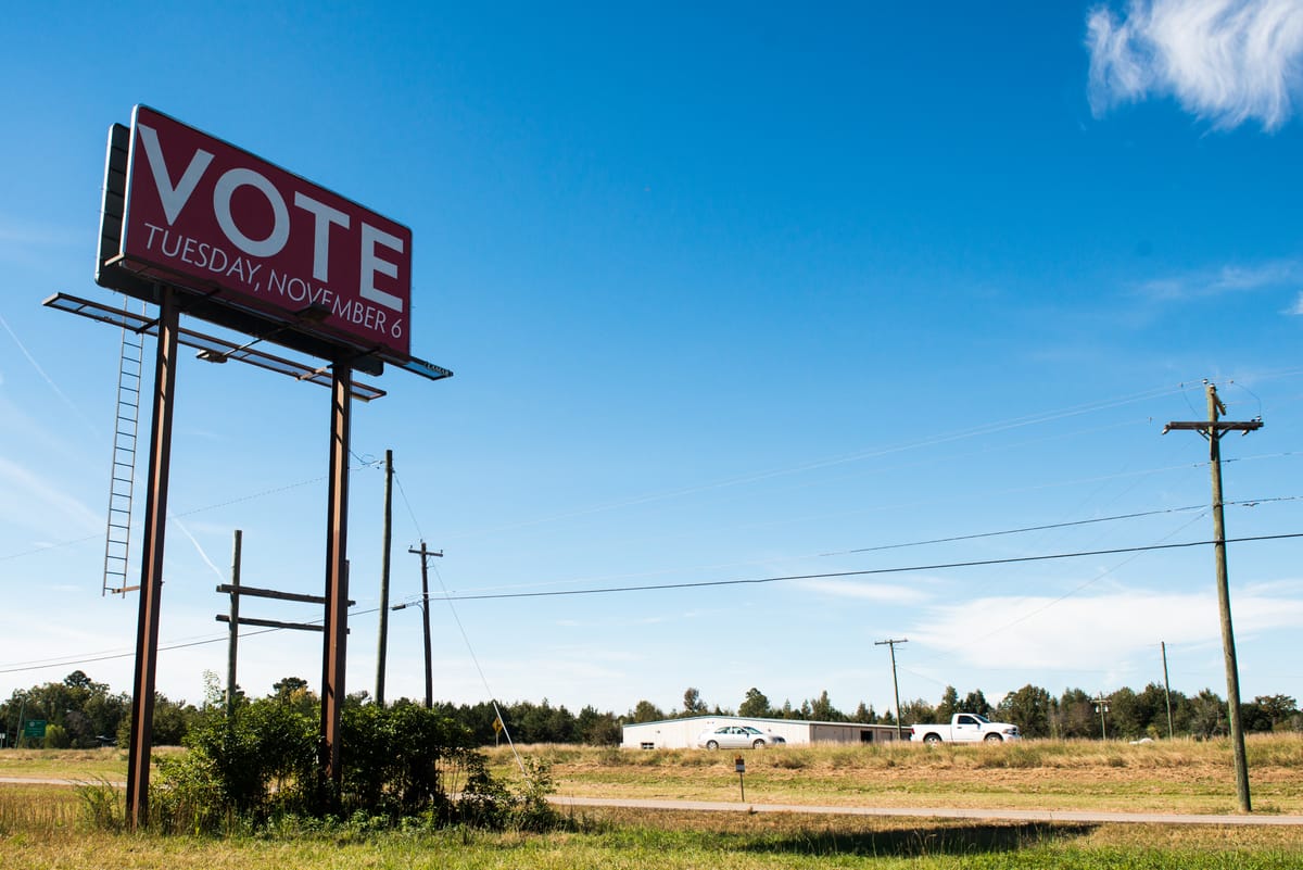
For the 2018 midterm elections, NCO purchased thousands of billboards across 10 regions aimed at increasing voter turnout by providing people with a reminder about Election Day. The billboards were non- partisan and contained a reminder to vote, the election date, and small organization logo (see Figure 1).

This report focuses on the billboard purchases in three elections across two regions: (1) the 2018 general election in Maricopa County, AZ where the election of note was Arizona’s U.S. Senate seat and (2) the 2018 general and runoff elections in Mississippi where the elections of note were two simultaneously open U.S. Senate seats. (See Table 1 for more details on the elections.)
These two regions are geographically and demographically different. Maricopa County, Arizona is home to the city of Phoenix and the Phoenix Metropolitan area (including Glendale and Scottsdale). It has a population of 4.4 million people and when the large desert area surrounding the metropolitan area is excluded, it is a highly developed urban and suburban space. Alternatively, the entire state of Mississippi has just under 3 million people living in it and its largest metropolitan area, Jackson, has a population of 540,000. Unlike Maricopa County, Mississippi is also home to smaller, more isolated towns.
The elections going on in these two regions in 2018 were also quite different. Maricopa County featured a very high-profile and close Senate race between Democrat Kyrsten Sinema (D) and Republican Martha McSally (R). Both campaigns were well-funded and there was considerable outside money spent in support of both candidates. Some or all of eight of the state’s nine congressional districts also overlap Maricopa county. None of the 2018 House races were particularly competitive. (The closest race occurred in District 1 where Tom O’Halleran (D) defeated Paul Babeu (R) by about 8%.)
The Mississippi general election was unusual in that it featured two Senate races at the same time. Incumbent Roger Wicker (R) defeated David Baria (D) in the state’s regularly scheduled Senate election. A second, concurrent special election was held to finish the term of Thad Cochran (R), who had retired. Cochran was replaced using a non-partisan top-two general election where the top vote-getter is elected only if they received more than 50% of the vote. Failing that, the top two vote-getters compete in a runoff election. The original 4-person race failed to produce a winner, so a runoff was held on November 27th where Cindy Hyde-Smith (R) defeated Democrat Mike Epsy (D). All three of these Mississippi races were significantly less high profile than the Arizona Senate race. In fact, the combined spending in all three Mississippi Senate races was only a fraction of that spent in the Arizona race.

Research Question & Analytical Approach
The research question is: What was the effect of NCO’s billboard program on voter turnout?
Like any GOTV effort, billboards exist in a variety of electoral contexts (national, state, and local) that impact turnout to varying degrees. The question of how effective billboards are at improving turnout is conditioned by these various contexts, including all the other GOTV efforts that may be going on in the election. Previous attempts to analyze the impact of billboards on voter turnout have not found significant effects.2 These efforts used a combination of individual-level and aggregate-level research designs. Individual-level research designs examine the likelihood a person turning out to vote while aggregate- level analyses examine the overall turnout in a given space (e.g. Census block group, voting precinct). While there are certainly trade-offs, an individual-level analysis is generally accepted to be the better approach as it allows for a more fine-grained examination of the factors at work. While all of the previous research conducted on billboard effectiveness appears to be of very high quality, the combination of different elections and alternative approaches used here could yield different conclusions.
An analysis of the effectiveness of billboards presents a variety of theoretical and empirical challenges, and the two cannot be divorced from one another. To begin, the hypothesis is that people that were exposed to (i.e. treated with) a NCO billboard turned out a higher rate than people who were not. But with exposure unknown, something must proxy for it. In this case, the most sensible proxy is distance to a billboard as a person living near a billboard is more likely to be exposed to it. Thus, the operating hypothesis is actually that, all else being equal, people who live close to a NCO billboard voted at higher rates than people who lived far away.
This distance-based proxy for exposure presents some problems. A considerable portion of the billboards purchased by NCO are along highways that route through more urban and suburban areas. Those living near these highway billboards (by road or as-the-crow-flies) may not actually be the people who are regularly exposed to it. Consider the image in Figure 2 below, which shows one of NCO’s Maricopa County billboard purchases. The billboard is located along West Maricopa Freeway but is primarily viewed from Route 60 (see inset). There are a considerable number of homes in this Central City South neighborhood that are spatially proximate to the billboard but the people who live in these homes are not the people most likely to see it. Indeed, the people who live closest to this billboard would need to travel to the closest highway exit and head in the direction of the billboard to see it. Meanwhile, people traveling from farther away may pass it every day on their commute. Previous research does not appear to have accounted for this challenge when using distance as a proxy for exposure.

Because distance is proxying for likelihood of treatment, the distinction between “effect” and “observable effect” is important. Any person that passes by a billboard may be reminded of when election day is and, as a result, vote (or not vote) – this would be an effect. However, absent the ability to track every person’s actual exposure, we are forced to look for what I will refer to as a spatially proximate observable effect. For this analysis that means identifying increased turnout near appropriate billboards. Highway billboards are not likely to have a spatially proximate observable effect for the reasons outlined above. A spatially proximate observable effect is more reasonable if the billboard is situated in a place where the people who live close to the billboard are also the people who are most likely to see it. These billboards tend to be the ones in commercial areas that have adjacent residential areas.
The core of my approach is to look for an effect in the places where we are most likely to be able to observe one. If there is a spatially proximate observable effect, then there is very likely also a more general effect that is not constrained to those living closest to a billboard (e.g. those who regularly pass a billboard on the highway during their commute to work) – but we do not have a good way of measuring the more general effect.
Billboard Coding
Central to this idea of a spatially proximate observable effect is that not all billboard locations should be treated the same. Thus, billboards needed to be broken down into those that were likely to have a spatially proximate observable effect and those that were not.4 Using pictures of the billboards from AdQuick and satellite images of each billboard location, I coded each billboard as (1) unlikely, (2) likely, or (3) very likely to have an spatially proximate observable effect. (A fourth category included those billboards for which a determination could not be made.) Purchases in Maricopa County also included 26 bus stop signs that were all coded as “unlikely”. Table 2 explains the coding scheme and provides examples. This coding process resulted in a substantial reduction in usable billboards while still leaving plenty to complete the analysis with (Table 3).


The Datasets and their Geography
To test the effect of the billboards I developed a Geographic Information System (GIS) and individual- level dataset for each of the three elections. Registered voters in both regions were geocoded using Catalist voterfile data and the Census Bureau’s Address Locator files. Match rates (the percent of registered voters that could be successfully geocoded) appear in Table 4 below. These match rates are high (the Maricopa rate is very high) and Zip Code analyses suggests that the unmatched addresses were mostly located in more rural areas where address data tend to be less accurate. These are also areas were NCO tended not to have billboards.

Billboard locations were also mapped and the direct distance (as-the-crow-flies) between each person on the voter list and all billboards within 5 miles (for Maricopa) and 10 miles (for Mississippi) were calculated.5 Geocoding also allowed each voter to be tied to a Census block group and associated Census data. The maps below (Figures 3 and 4) show the geographic distribution of signs for the two regions. The Mississippi County maps combine the billboard purchases for the two elections (108 billboards were purchased in both elections).


Making Appropriate Comparisons
NCO’s billboard purchases were not made randomly. In purchasing billboards, NCO was constrained by budget and AdQuick’s availability, and then prioritized the selection of billboards in minority and lower-turnout areas. Even without those constraints there is no reason to believe that billboards are randomly distributed across the regions being analyzed – which would be ideal for analysis. While complete datasets are available for both Maricopa County and Mississippi and some controls for the non-random placement of billboards could be instituted, my primary approach is to constrain the analysis to areas around the billboards that NCO purchased. As such, I constrain the datasets to all registered voters living 5 miles from a billboard in Maricopa County and 10 miles from a billboard in Mississippi. The difference in radii is due to Maricopa County having a significantly higher population density than the state of Mississippi. This analysis compares people that live close to a NCO billboard with those that live farther from a NCO billboard, but still within the given radius. I also use a ring analysis that expands the pool of examined voters beyond the radial thresholds to further empirically validate the results – this is discussed in more detail below.
Estimating the effect of the distance to a billboard on turnout necessitates controlling for other potential causes of turnout (if those causes are correlated with distance). For simplicity and comparability, I utilize Catalist’s 2018 voter propensity score. This is a modeled measure coded 0 to 100 that incorporates data on vote history, age, race, household participation, and address certainty. Pearson’s R correlations (see Table 4) indicate that it is highly correlated with turnout (0 = unrelated; 1 = perfectly related). NCO may also wish to use the Catalist measure as a tool for making billboard purchasing determinations in the future; using it here allows for the models to be consistent with that future purchasing strategy.

The distance analysis that I present below is based on Logit regressions that are appropriate for estimating individual level turnout. Existing GOTV research points to mid-propensity voters being the most reactive to GOTV efforts. To account for this, I break people up into propensity groups and then estimate separate models for each group while also controlling for propensity in the models. Tables 6 describes the in-radius turnout rate for each propensity group and Table 7 provides the in-radius number of voters for each propensity group. I exclude high-propensity voters from the analysis because of their extremely high turnout rates – it is unlikely that the NCO billboards are significantly impacting them.
For the two general elections being analyzed, I also control for congressional district competitiveness (via fixed effects). In the Maricopa County analysis, I include indicators of whether the person registered as a Republican or a Democratic (as opposed to as an Independent or some other party). This is not an option for the Mississippi analysis as Mississippi has non-partisan voter registration. Finally, the models all contain Census block-level turnout in the 2016 election. The Catalist voter propensity score is entirely based on individual-level data and does not include any spatial-contextual information. This spatial- contextual turnout variable helps to further control for the many non-billboard neighborhood factors that may drive turnout (e.g. polling place issue, neighborhood norms, the presence of local community activists, etc.).

Distance Analysis
I ran two versions of each analysis. The first version includes everyone who lived within the radius of a billboard that I coded as “likely” or “very likely” to have a spatially proximate observable effect. The second version is restricted to only people who live within the radius of a billboard that I coded as “very likely” to have a spatially proximate observable effect. Recall that the goal is to try to find an effect in the places where one is most likely to be seen. The “very likely” billboards were the ones determined prior to analysis as having the most potential to do so.
Below, I summarize the results and then present a visualization that further clarifies the effect of the billboards. That visualization is followed by a discussion of additional conclusions that can be drawn from the results.
Mississippi – Summary of Results
- Living closer to a NCO appears to have caused a slight boost in the chance that a person voted in the Mississippi general and Mississippi runoff elections.
- The effect of the NCO billboards was a bit stronger in the Mississippi runoff than it was in the Mississippi general.
- There was a positive effect on turnout for both low and moderate propensity voters. However, the effect for low propensity was limited to the Mississippi general election.
- There was not a substantial difference between the voters who lived near a billboard that I coded as “very likely” to have a spatially proximate observable effect, rather than just “likely”.
Maricopa County, AZ – Summary of Results
- With one important exception, living close to NCO billboard does not appear to have impacted turnout in the Arizona election in Maricopa County.
- The exception is that low-propensity voters in Maricopa County who lived close to a billboard I coded as “very likely” to have a spatially proximate observable effect, were slightly more likely to have voted than a low-propensity voter who lived farther away.
The graph that follows (Figure 5) shows the probability of turnout given a person’s proximity to a NCO billboard, holding the other variables in the model – namely, vote-propensity – constant. (The graph only contains lines for the models that had the desired effect.) The solid lines indicated the estimated probability and the dotted lines indicate the uncertainty of that estimate. The downward slope of the lines can be read as indicating that people who lived close to a billboard voted at a (slightly) higher rate than people who lived farther away. For example, a moderate propensity Mississippi voter living right near a NCO billboard was about 2.5 percentage points more likely to have voted in the runoff than a voter living 10 miles away. Similarly, a low propensity Maricopa County voter living right near a billboard was about 2.3 percentage points more likely to have voted than someone living 5 miles away.

The effect of distance is probably not as linear as this graph suggests. The distance measure is an imperfect measure of exposure and the effect likely dissipates at an accelerating rate as distance increases. (The ring analyses in the following section help to clarify this point.) With that in mind, I think it is wise to avoid reading too much into specific probabilities at specific distances. Rather, I interpret the results as a preliminary overall indicator that those who were likely to be exposed to the NCO billboards were slightly more likely to have voted than those who were less likely to be exposed to the NCO billboards. And given that a spatially proximate effect was identified, it is reasonable to conclude that there is a non-spatially proximate effect too. Put differently: even though this analysis excluded billboards along the highway and other similar locations, highway billboards probably had an impact on turnout as well – it is just not an effect that can be easily seen.
Beyond the general findings presented above, these results suggest some additional conclusions about the effectiveness of NCO’s billboard program. Foremost, the strength of the results increases as the salience of the election decreases. The Mississippi results are stronger than the Maricopa County results and the Mississippi runoff results are stronger than the Mississippi general results. There is a good theoretical explanation for this: less noisy elections allow the billboards to stand out more. Arizona had a a high profile, highly funded election in 2018 that garnered a lot of national attention and money. The Mississippi elections were salient (indeed, turnout was quite high) but received less media and financial attention than Arizona. And the Mississippi general was the focus of more national attention than the runoff. The runoff was also conducted on an atypical election day and only had one election on the ballot. It is difficult to know whether the election noise obscured the ability to see the effect of billboards or actually eliminated it altogether. As discussed in more detail below, future analyses may benefit from research designs that allow for additional exploration of this theory.
I also did not find substantial differences between the models that combined billboards that I coded as “likely” and “very likely” to see a spatially proximate observable effect and the models that strictly looked at “very likely” billboards. At the same time, the “very likely”-only models do contain the only significant effect for the Maricopa County analysis. My coding does appear to be producing some distinctions, but they are fuzzy. This points to the need for a more reliable (probably multi-person) coding regimen.9 Relatedly, the low-propensity results are worth highlighting because previous research has found that lower-propensity voters tend to be less susceptible to GOTV efforts. If these results hold up to future analysis, it would indicate that billboards are a good way to boost turnout among these potential voters.
Ring Analysis
The distance analysis presented above offers evidence that those who lived close to a NCO billboard were slightly more likely to have voted than those who live farther away from a NCO billboard, but within a given radius. In constraining the analysis to only those potential voters that live within a given radius of a billboard, I guard against some of the challenges of analyzing a non-random selection of billboards. However, this constraint may also cause some problems. Primarily, everyone in the analysis has a reasonable chance of being exposed to a NCO billboard. The ring analysis I present below offer an opportunity further support those results by introducing people that live far away from billboards into the pool. I focus this ring analysis on the three groups/models that presented the most promising results in the distance analysis: (1) moderate-propensity voters in the Mississippi general, (2) Moderate- propensity voters in the Mississippi runoff, and (3) Low-propensity voters in the Maricopa County election that live near a billboard I coded as very likely to have a spatially proximate observable effect.

In this analysis I compare people that live within a specified radius of a billboard with those that live far away from any billboard coded as “likely” or “very likely”.10 For example, I compare those that lived within 1 mile of a NCO billboard in the Mississippi general with those that lived at least 10 miles from a billboard (in doing so, excluding everyone who lives between 1 and 10 miles). I then repeat this for increasingly larger rings – up to 5 miles for Maricopa county and up to 10 miles for Mississippi. Figure 6 above shows this comparison for a 2-mile ring. The reason I exclude those living between the ring and the far radius is that if they are impacted by the billboards as the distance results suggests, then it is wise to avoid them as a comparison. Put differently, I compare those that were potentially exposed with those that were unlikely to be exposed. With each iteration I theoretically dilute the pool of voters that could be impacted by a billboard. To do this, I estimate the exact same models that I estimated in the distance analysis but replace the distance variable with one that indicates whether a person lives inside the ring (1) or far away (0).
I am looking for two things in these analyses. First, I am looking to see if, all else being equal, those who live within the ring voted at a higher rate than those who lived far away. And second, I am looking to see if the effect dissipates as the ring grows in size. As you will see in Figures 6 and 7 this is what I find. As with the previous graph, the solid line represents the estimate and the dotted line represents the confidence in that estimate. Specifically, the lines indicate the increase in the probability of a person that lives in the ring voting versus a person that lives far away. In the Mississippi runoff election, for example, all else being equal, a registered voter living within 2 miles of a NCO billboard was 2.3 percentage points more likely to have voted than someone who lived at least 10 miles from any NCO billboard. The marginal gain of a billboard for turnout decreases as the pool of voters surrounding it expands outward. For the most part, the graphs indicate that the effect of the NCO billboard is strongest when looking strictly at those who live within a few miles of a billboard. These ring analysis results add support to the distance analysis results by showing a similar outcome using a different comparison. But as with the previous analysis, I believe the best way to read the results is as an overall indicator that the billboards have a slight positive effect on proximate turnout.


A Word of Caution
It is important to note the results presented here are subject to some important caveats and definitive conclusions should not be drawn from them. Foremost, the large-N of individuals included in the analysis may lead to statistically significant results for most variables in the model. A natural trend in the data unrelated to billboard proximity but incidentally correlated with it will likely be significant, even if the magnitude of that relationship is very weak. Seeing similar results in other regions would reduce this concern. Secondly, these models are somewhat sensitive to their specification. For example, when variables for race, age, and gender substitute for the Catalist voter propensity measure in the distance models, the relationships tend to weaken and/or become insignificant.11 And third, there may be omitted variables (i.e. not available) that correlate with proximity to billboard and turnout that would change the results. More definitive conclusions are going to require additional research.
Avenues for Future Research
This report has offered evidence that NCO’s billboard program in Mississippi had a small positive effect on voter turnout. Evidence of such an effect is weaker for NCO’s Maricopa county program. The differing results for Mississippi and Maricopa County strongly indicate that additional research is necessary to make more definitive conclusions about the effectiveness of billboard GOTV strategies. There are three separate avenues for future research that NCO may wish to consider. The first is an expansion of the analysis presented here. The second involves analysis of other regions in the 2018 program. And the third involves making future billboard purchases with an experimental research design in mind.
In finding some evidence that a turnout effect exists, additional analysis of both Maricopa County and Mississippi (and/or other regions) could focus on better identifying the characteristics of billboard locations that enhance turnout. This could be helpful in deciding which billboards to buy in future elections. The coding process instituted for this analysis was fairly quick, and involved only me. To better understand which billboards are most effective, a more detailed process would need to be instituted where each billboard purchased was coded for various attributes (e.g. population density, types of homes that are nearby, how commercial or residential the area is, the ability of people to clearly see the billboard, proximity to universities, and others). Such a coding process would take advantage of additional GIS data and use multiple coders and inter-coder reliability tests.
If NCO would like to continue to further validate the findings of the research presented here prior to the next round of billboard purchases, analyses of other 2018 regions could be instituted. Analyses could focus on areas that NCO has a particular interest in or could focus on less-salient elections where it is probably more likely that there will be results indicating the billboards boosted turnout. This research could also utilize a more detailed coding process like the one described above.
To more conclusively validate the results in this analysis, a research design that begins with the purchasing process is needed. There are multiple different research designs to consider but one potentially fruitful one would be to randomly select billboards from the available pool – ignoring all locational characteristics (e.g. past turnout, race, ethnicity, etc.). This in and of itself would likely improve the generalizability of the results. However, the randomly selected billboards could then be randomly assigned to a control group – for which billboards are not purchased or billboards are left blank – and a treatment group where billboards contain a reminder to vote. Turnout for billboards in the control group would be compared with turnout in the treatment group. If NCO is interested in trying out the effectiveness of different billboard language or designs, additional experimental groups could be utilized.
Final Takeaways
This analysis of Mississippi and Maricopa County suggests that NCO’s billboard program is worth continuing if NCO is satisfied with the potential turnout gains. Given the challenges of getting people to open letters and read emails, billboards offer a GOTV strategy with high potential to actually reach the people that drive near them. Continuation is also justified by the evidence that billboards may boost turnout among historically difficult to reach low-propensity voters.